Getting data from one table to another in Excel is an important part of managing and processing information. From using basic functions like VLOOKUP, HLOOKUP, MATCH function with INDEX function to advanced tools like Power Query. The following article will guide users on how to make the most of this tool, making it easier to move data between tables.
Nội dung
I. What is moving data from one table to another?
Getting data from one table to another is the process of copying or moving information from one location to another within the same Excel file.
This is an important and useful trick in organizing and processing data, allowing users to rearrange information according to specific usage needs.
II. How to Get Data from One Table to Another in Excel
This article will guide you through the 3 simplest and fastest ways to transfer data from one table to another, helping users take advantage of all the capabilities of Excel during their work.
1. How to use the VLOOKUP function
The VLOOKUP function is a powerful tool that searches and retrieves data in a table based on a specific key value and returns the related value in another column. Mastering how to use this function will enhance your data processing capabilities.
The formula for the VLOOKUP function is: =VLOOKUP(lookup_value, table_array, col_index_num, [range_lookup]) , with the following components:
- Lookup_value: The value to search for.
- Table_array: The data range that contains the value to find. This range must have at least 2 columns. Use the F4 key after selecting the range to freeze it.
- Col_index_num: The column number in the search range that contains the value to return.
- Range_lookup: The search method. Set range_lookup to 0 or FALSE for exact search; to 1 or TRUE or leave it blank for approximate search.
Example Table Structure: Here’s a simplified version of the Year-End Summary Table for reference:
| Student ID | Name | Final Score (%) | Letter Grade | GPA |
|---|---|---|---|---|
| 1 | John Smith | 93 | A | 4.0 |
| 2 | Emily Davis | 85 | B | 3.0 |
| 3 | Michael Brown | 78 | C | 2.0 |
| 4 | Sophia Wilson | 91 | A | 4.0 |
| 5 | James Johnson | 88 | B | 3.0 |
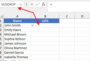
We have 2 sheets, sheet 1 is named Year End Summary Table, sheet 2 is named GPA. The task is to transfer data from Sheet 1 to sheet 2 to look up the GPA of students using the vlookup function.
How to do:
Step 1: In the cell where the result needs to be displayed, press “=”, show the item in the corner of the table, select “Vlookup”.
Step 2: After selecting “Vlookup”, the following table appears, fill in all the information in the table and press OK
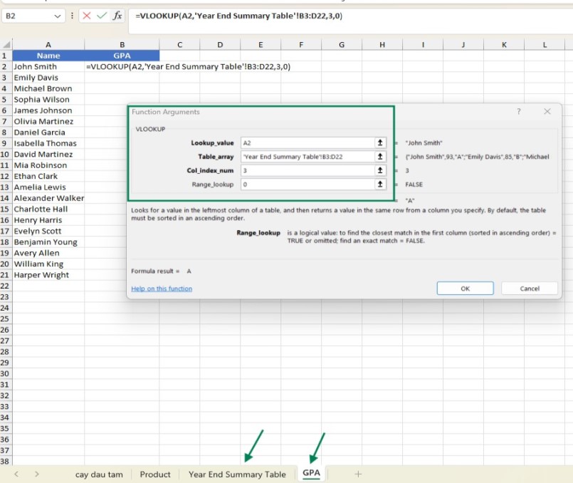
Step 3: Return GPA results of students from sheet 1
2. How to use the HLOOKUP Function
The HLOOKUP (Horizontal Lookup) function is a tool used to search for a value in a horizontal row of a data range and then return the corresponding value from that row.
This function works similarly to VLOOKUP, but instead of searching vertically, it searches horizontally. This method is especially useful when working with horizontally arranged data tables.
The syntax of the HLOOKUP function is: =HLOOKUP(value, table, row_index, [range_lookup]) , with the following components:
- Value: The value to look up to match in the first row of the table.
- Table: The table containing the data to be searched.
- Row_index: The row number in the table containing the data to be searched.
- Range_lookup: The search method. Set range_lookup to 0 or FALSE for exact search; to 1 or TRUE or leave it blank for approximate search.
Example Table Structure: Here’s a simplified version of the Year-End Summary Table for reference:
| Name | John Smith | Emily Davis | Michael Brown |
| Final Score (%) | 93 | 85 | 78 |
| Letter Grade | A | B | C |
| GPA | 4 | 3 | 2 |
3. How to combine the MATCH and INDEX functions
The MATCH function is a powerful tool for determining the position of a specific value in a data range. It is not a method of returning data, but only determining the position of that data. This function is suitable when working with a small amount of data, within a limited range, and requires the location of data to be determined quickly.
The MATCH function is often used in conjunction with the INDEX function, forming a powerful pair of tools that overcome some of the limitations of the VLOOKUP function.
The formula for the MATCH function is: =MATCH(lookup_value, lookup_array, [match_type]) , with the following specific components:
- Lookup_value: The value to look up.
- Lookup_array: The range of data that contains the value to look up. This range must have 2 or more columns.
- Match_type: Search type. Use 0 for exact match, 1 or nothing to find the position of the value less than or equal to the search value, -1 to find the position of the value greater than or equal to the search value.
The formula for the INDEX function is: =INDEX(array, row_num, [column_num]) , with the following elements:
- Array: The range of data to search.
- Row_num: The row number in the data range that contains the value to extract.
- Column_num: The column number in the data range that contains the value to extract.
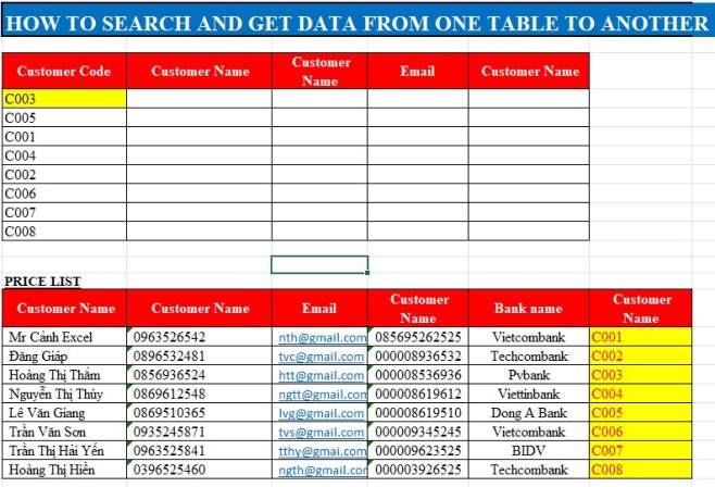
For example: We have a table as shown below
The problem is to extract data from the “PRICE LIST” table to the “Customer Name” column in the table above.
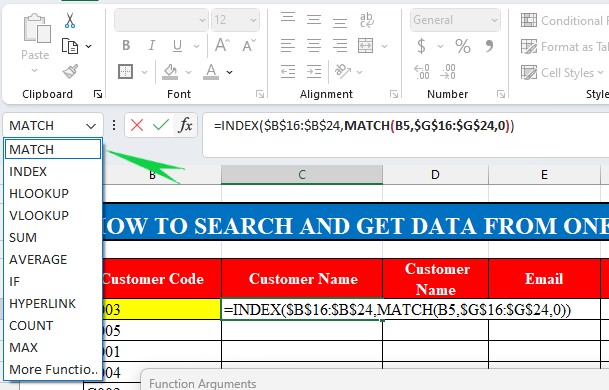
Step 1: In the “Customer Name” section, enter “INDEX function“, the “Function Arguments” table will appear.
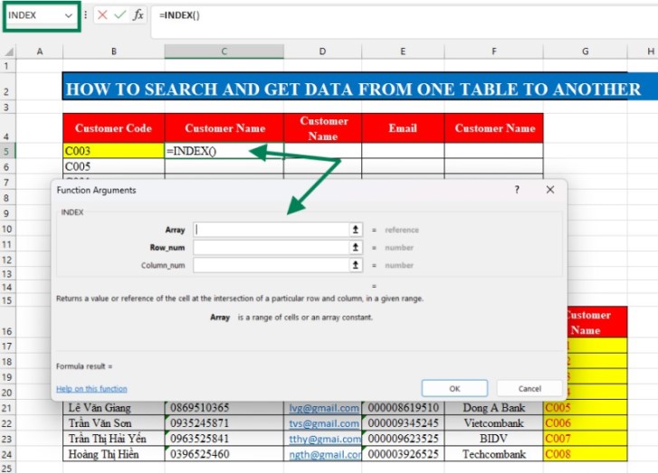
Step 2: Fill in the information in the “Array” fields
Step 3: Click on the MATCH function and Fill in the information in the fields, click OK and you’re done.
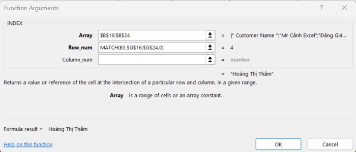
Note: After completing step 3, the INDEX function input table will now look like this:
In the Column_mun field, you do not need to fill in the information, the data will still give accurate results. This field is not required.
Above are the 3 detailed ways to transfer data from one table to another in Excel. I hope this article helps you in your work and studies. If you have any suggestions, feel free to leave a comment below, and don’t forget to share if you find it helpful.
See more: 4 Ways to set a password for Excel files: avoid editing and copying