When entering a large amount of data, it can be time-consuming and may lead to errors such as duplicate entries. Therefore, creating a drop down list in Excel helps you quickly create data lists. Let’s explore how to create, add, and delete Drop Down lists in Excel Online with Lammocofficeatoz.
Nội dung
I. What is a Drop Down List?
A Drop Down list is a method of creating a pull-down selection of different data values in a blank cell in Excel. Drop Down lists are widely used because they help control the values entered into a cell.
Some benefits of Drop Down lists include:
- Creating specific categories within a single blank cell.
- Reducing duplicate or misspelled information.
- Usable for various purposes and industries (inventory management, attendance tracking, location classification, etc.).
II. How to Create a Drop Down List in Excel
You can create a Drop Down list in Excel using different methods. Below are three ways to create a Drop Down list.
1. Creating a Drop Down List Manually
If you want a simple option in a drop down list within a blank cell, the quickest method is manual entry.
Steps:
Select a cell or range where you want to create the Drop Down list.
Go to the Data tab → Select Data Validation in the Data Tools group.
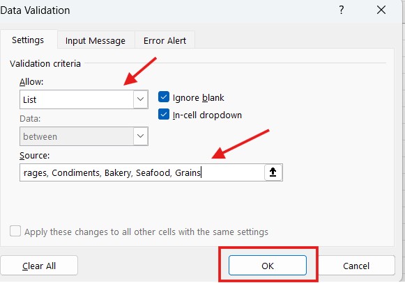
In the Data Validation window, under Settings:
Select List as the validation criteria.
In the Source field, enter the desired options, separated by commas.
Click OK to complete.
2. Creating a Drop Down List Using Cell References
Another method allows you to create a Drop Down list by using a range of cells as the data source.
Example:
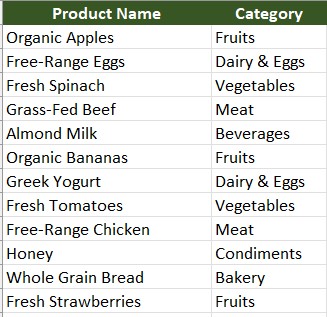
We want column B in the “Inventory Management” sheet to display a Drop Down list of all fabric types in stock. The source data, including fabric names and quantities, is stored in another sheet named Source within the same Excel file.
Steps:
Prepare a source data table, which can be in the same sheet or another one. In this example, we enter data in A1:A6 on a separate sheet named Source.
Select the target cell or range where you want to create the Drop Down list.
Go to the Data tab → Click on Data Validation.
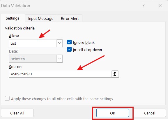
In the Data Validation window, under Settings:
Select List as the validation criteria.
In the Source field, enter the reference range from the Source sheet.
Click OK to complete.
This method creates a Drop Down list where each item appears as a separate entry in the Drop Down menu.
3. Creating a Drop Down List Using the OFFSET Function
You can also use the OFFSET function to create a dynamic Drop Down list that automatically updates when new items are added at the end of the list.
Formula:
=OFFSET(reference, rows, cols, [height], [width])
In the OFFSET function:
- reference: The starting cell or range.
- rows: The number of rows to move from the reference.
- cols: The number of columns to move from the reference.
- height (optional): The number of rows to return.
- width (optional): The number of columns to return.
Example:
We will use OFFSET to create a dynamic Drop Down list.
Steps:
- In the “Inventory Management” sheet, select the cells where you want the Drop Down list (e.g., B2:B7).
- Go to the Data tab → Click on Data Validation.
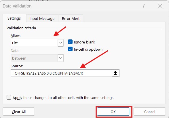
- In the Data Validation window, under Settings:
- Select List as the validation criteria.
- In the Source field, enter the following formula:
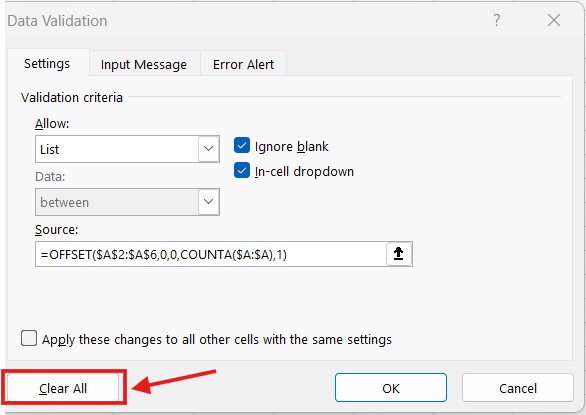
=OFFSET($A$2:$A$6,0,0,COUNTA($A:$A),1)
Explanation:
The formula starts at A2 in the Source sheet.
0,0 keeps the reference at the same row and column.
COUNTA($A:$A) counts the number of non-empty cells in column A, ensuring the Drop Down list updates automatically when new items are added.
1 sets the width to one column.
Click OK to complete.
This method allows the Drop Down list to update automatically whenever new data is added to the source list.
III. How to Edit an Existing Drop Down List in Excel
1. Allowing Other Entries in a Drop Down List
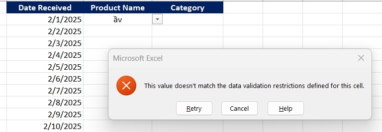
Once a Drop Down list is set up in your worksheet, those cells will only accept values that are part of the list. If you try to enter a value that is not included in the created Drop Down list, you will receive an error message, as shown below:
To allow users to enter values that are not in the source list, follow these steps:
Steps:
Select the cell(s) containing the Drop Down list where you want to allow additional entries.
Go to the Data tab → In the Data Tools group, select Data Validation.
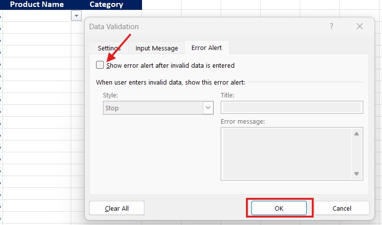
In the Data Validation window, go to the Error Alert tab and uncheck the box Show error alert after invalid data is entered.
Click OK.
Now, you can enter any value in the Drop Down list cell without receiving an error message.
2. Adding Items to a Drop Down List in Excel
Even if you are not using a dynamic Drop Down list, this simple trick allows you to quickly add new items to an existing Drop Down list.
Steps:
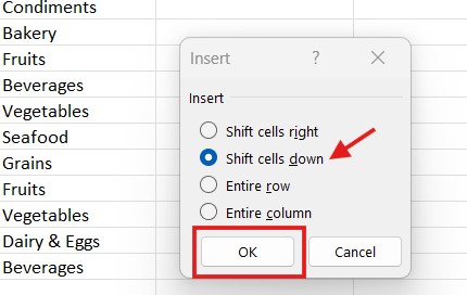
In the source list, right-click on the blank cell where you want to add a new value.
Select Insert → Click Shift cells down → Click OK.
Enter the new value in the blank cell that was just created.
Excel will automatically expand the source range in your data table to include the first and last values in the Drop Down list.
3. Removing Items from a Drop Down List in Excel
To quickly remove an item from a Drop Down list, follow these steps:
Steps:
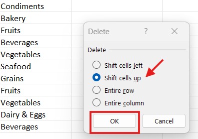
Go to the source list and right-click on the value you want to remove.
Click Delete → Select Shift cells up.
Click OK.
Now, the Drop Down list cells in the worksheet will be updated to reflect the adjusted source data range.
IV. How to Remove a Drop Down List in Excel
Steps to Remove a Drop Down List:
- Select the entire range where the Drop Down list is applied. Then, go to the Data tab on the toolbar and click on Data Validation in the Data Tools group.
- The Data Validation dialog box will appear. Click Clear All, then click OK to confirm.
- Excel will remove the Drop Down list, but the existing data in the cells will remain unchanged.
V. Some Notes on Creating Lists in Excel
Creating lists in Excel is an essential skill for organizing and managing data effectively. However, to ensure that the list functions well and can be easily modified, you should keep the following points in mind:
1. Ensure Data Accuracy
The data in the list must be accurate and consistent. If the list contains unnecessary duplicate values or inconsistent formats (such as mixing numbers and text in the same column), it may cause difficulties when using it.
Example: A product list should only include items like “Laptop, Phone, Tablet” instead of unrelated values such as serial numbers or notes.
2. Use the Appropriate Data Format
Make sure the columns in the list are formatted correctly. If the list contains numerical data, you should set the column format to Number to facilitate calculations. If the list contains text, format the column as Text to prevent Excel from automatically converting the data.
Example: If the list contains dates, format it as Date so Excel can interpret it correctly and support filtering or calculations.
3. Use an Easy-to-Remember Named Range
When using a Named Range to define a list, choose a short, easy-to-understand name without special characters. This makes it easier to use in formulas or references in other parts of the worksheet.
Example: Name it ProductList instead of a long name like New_product_list_data.
4. Avoid Changing the Data Structure
After creating a list, avoid inserting or deleting columns unless absolutely necessary, as this may disrupt formulas or related references. If you need to add columns or rows, check and update the formulas or reference sources to prevent errors.
5. Use Tables to Manage Lists
Converting a list into a Table helps you manage it more easily and allows the list to expand automatically when new data is added. Tables also provide useful features such as filtering, sorting, and consistent formatting. To do this, select the list, go to the Insert tab, and choose Table.
6. Keep the Drop List Data Source Fixed
When creating a Drop Down list, ensure that the data source is placed in a fixed location or use a Named Range. Otherwise, changing the position or content of the source data may cause the Drop List to malfunction or lose data.
Example: If the Drop List references Sheet2!A1:A5, it’s better to define a fixed range or name it SourceList for easier management.
7. Avoid Unnecessary Gaps
Data in the list should be entered continuously, without empty rows or columns in between. This helps Excel accurately determine the data range and improves support for functions like filtering or calculations.
8.Check for Errors After Creating the List
After creating a list or a Drop Down list, check to ensure it functions as expected. Try selecting each item in the Drop List or review the formulas if the list is used in calculations. If errors occur, you can adjust the source data or check the Drop List settings in Data Validation.
VI. Frequently Asked Questions About Creating Lists in Excel
1. Can I create a Drop List using data from another Excel sheet?
Yes. You can create a Drop Down list using data from a different sheet or even another Excel file. The best way is to use a named range for the source data. This keeps the list functional even if the source data moves.
To create a dynamic list that updates automatically when data changes, use formulas like OFFSET hoặc INDEX. This ensures the Drop List reflects any additions or removals without manual updates.
2. Can I enter a value that is not in the Drop List?
By default, Excel restricts entries to predefined values in the list to minimize errors. However, you can allow additional entries by adjusting the Data Validation settings:
- Uncheck “Ignore Blank” or enable input modes for free-text entries.
- For controlled flexibility, apply validation formulas to highlight values not in the list, ensuring consistency while allowing new inputs.
Conclusion
In this article, we have provided a comprehensive guide on how to use and create Drop down list in Excel using different methods. We hope that the information shared today has given you another useful tip for your work. If you find this article helpful, please share it with more people to spread the knowledge.
Wishing you success!
See more: Formula to Find Special Characters in Excel (Complete Guide)