How to use MATCH Function in Excel (examples and function combinations)

1

When learning Excel, users often use many different functions to calculate or search for specific data. In this article, we will share insights on how to use MATCH function in Excel. So what is the MATCH function? Let’s explore the details below.

I. What is the MATCH Function in Excel?

The MATCH function in Excel is used to find the position of a value within a data range. It then returns the exact position of that value within the range. By using the MATCH function, users can quickly locate the values they need, saving time compared to manual data searching in Excel.

II. Syntax of the MATCH Function in Excel

The syntax of the MATCH function is:
=MATCH(lookup_value, lookup_array, [match_type])

Where:

• lookup_value: The value to search for in the lookup_array. This can be a number, text, logical value, or a cell reference to one of these. This argument is required.
• lookup_array: The range or array to search within. This is also required.
• match_type: The type of match to perform. This argument is optional.

1. Types of Match in the MATCH Function

There are three types of match you can use:

1 or omitted (Less than): The function finds the largest value that is less than or equal to the lookup_value. The lookup_array must be sorted in ascending order.

0 (Exact Match): The function finds the first value that exactly matches the lookup_value. The lookup_array can be in any order.

-1 (Greater than): The function finds the smallest value that is greater than or equal to the lookup_value. The lookup_array must be sorted in descending order.

2. Notes When Using the MATCH Function

The MATCH function returns the position of the lookup value within the lookup_array, not the value itself.

The search is case-insensitive for text values.

If the lookup value is not found, the function will return an error.

When using match_type as 0 and searching for text, you can use the following wildcards:

• * (asterisk) to represent any sequence of characters.
• ? (question mark) to represent any single character.
• To search for an actual asterisk * or question mark ?, precede them with a tilde ~ (e.g., ~* or ~?).

If you do not specify the match_type, Excel will assume the default value of 1.

III. How to use the MATCH function in Excel

Here are the different types of MATCH functions in Excel:

Example Data Table:

No	Product Code	Product Name	Category	Price (USD)	Stock Quantity
1	A106	Orange Juice	Beverage	1.25	15
2	A109	Watermelon	Fruit	1.17	10
3	A105	Fresh Milk	Beverage	1.04	20
4	A107	Mango	Fruit	0.92	35
5	A101	Apple	Fruit	0.83	50
6	A104	Tomato	Vegetable	0.75	40
7	A102	Banana	Fruit	0.63	30
8	A103	Carrot	Vegetable	0.5	25
9	A110	Yogurt	Beverage	0.5	50
10	A108	Potato	Vegetable	0.42	45

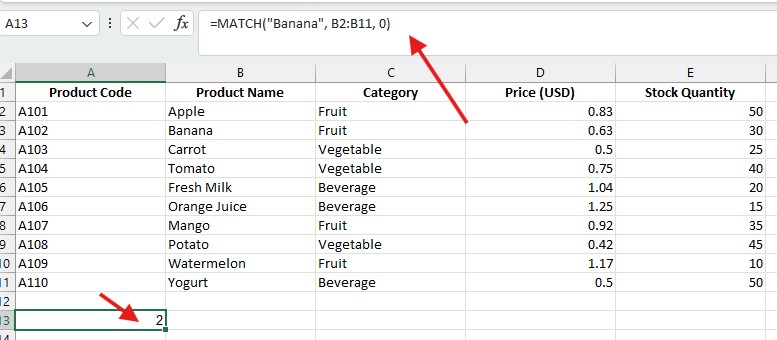
1. Exact Match (match_type = 0)

An exact match means the lookup value must be an exact 100% match with one value in the list. If not found, the function returns an #N/A error.

Formula:
=MATCH("Banana", B2:B11, 0)

Result: 3 (Because “Banana” is in the 3rd position of the range B2:B11). If “Banana” is not in the list, the formula will return #N/A.

2. Approximate Match (match_type = 1 or -1)

Approximate match means that the MATCH function will find the closest value that satisfies the condition:

• If match_type = 1 → Finds the largest value less than or equal to the lookup value (the list must be sorted in ascending order).
• If match_type = -1 → Finds the smallest value greater than or equal to the lookup value (the list must be sorted in descending order).

Approximate Match with match_type = 1 (find the closest value less than or equal to the lookup value, requires ascending order)
Suppose you want to find the approximate match for 0.8 in the price column.

Formula:

=MATCH(0.8, E2:E11, 1)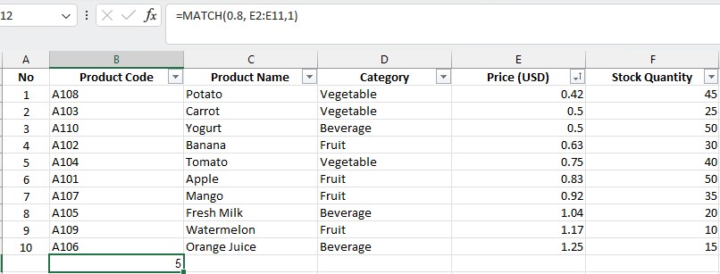 

Result: 5 → Corresponds to the price of Tomato (0.75).
Since 0.83 (Apple) is higher than 0.8, MATCH selects the closest smaller value, which is 0.75.

Approximate Match with match_type = -1 (find the closest value greater than or equal to the lookup value, requires descending order)
Suppose you want to find the approximate match for 1.1.

Formula:

=MATCH(1.1, E2:E11, -1)

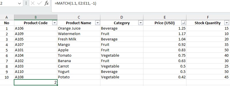
Result: 2 → Corresponds to the price of Watermelon (1.17).
Since 1.04 (Fresh Milk) is less than 1.1, MATCH skips it and selects 1.17 as the closest greater value.

Note:

• 1 requires the list to be sorted in ascending order.
• -1 requires the list to be sorted in descending order.
• If the sorting rule is not followed, the result may be incorrect or return an #N/A error.

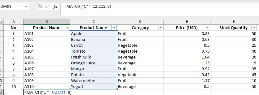
3. Wildcard Match (match_type = 0)

Wildcard match allows flexible searching within the list using special characters:

• * → Represents any sequence of characters.
• ? → Represents any single character.

Example (Using *)
=MATCH("C*", C2:C11, 0)
Result: 3 (Because “Carrot” starts with “C”).

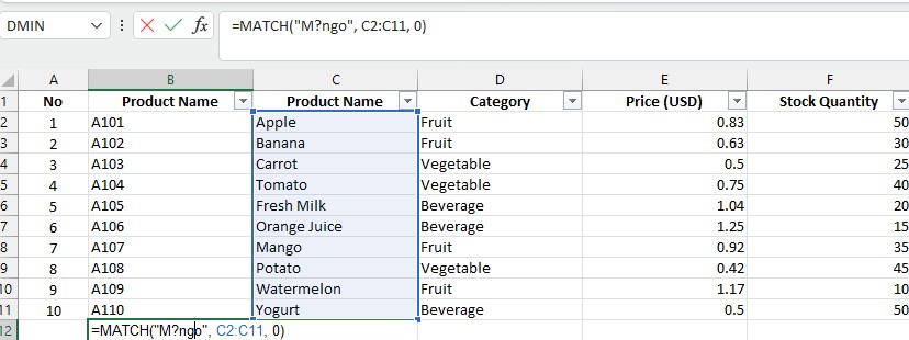
Example (Using ?)
=MATCH("M?ngo", C2:C11, 0)
Result: 7 (Because “Nho” matches the pattern “M?ngo“).

Note:

• Wildcards only work when match_type = 0.
• Not applicable for numeric data.

IV. Functions commonly combined with the MATCH function

MATCH is often used in conjunction with other functions to enhance lookup capabilities. Below are four popular functions that work well with MATCH, along with explanations and examples based on the data set above.

1️⃣ INDEX + MATCH 

The INDEX function retrieves a value from a specified row and column within a range.

Why combine INDEX with MATCH?

• MATCH helps find the row number dynamically, instead of using a fixed number.
• Unlike VLOOKUP, which only searches from left to right, INDEX + MATCH can search in any direction.

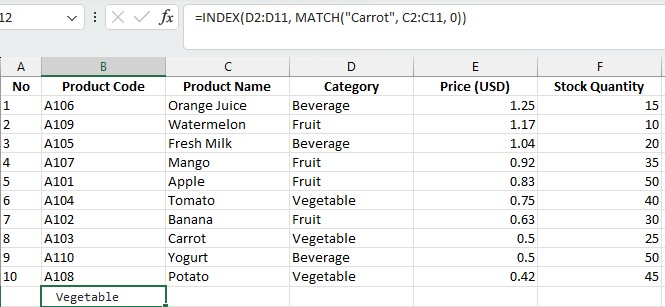
Example: Find the category of “Carrot”

=INDEX(D2:D11, MATCH("Carrot", C2:C11, 0))

Explanation:

• MATCH("Carrot", C2:C11, 0) finds the position of "Carrot" in the Product Name column (3rd row).
• INDEX(D2:D11, 3) returns the value from the Category column in the 3rd row → "Vegetable".

Result: "Vegetable"

2️⃣ VLOOKUP / HLOOKUP + MATCH

Why use MATCH with VLOOKUP?

Normally, VLOOKUP requires a fixed column index. If columns shift, the formula breaks. Using MATCH makes the column index dynamic.

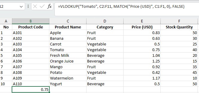
Example: Find the price of “Tomato”

==VLOOKUP("Tomato", C2:F11, MATCH("Price (USD)", C1:F1, 0), FALSE)


Explanation:

MATCH("Price (USD)", C1:F1, 0) → Identifies the position of the “Price (USD)” column within the header range C1:F1.

“Price (USD)” is located in the 3rd column of the range C1:F1.

VLOOKUP("Tomato", C2:F11, 3, FALSE) →

• Searches for “Tomato” in the first column of the range C2:F11 (the “Product Name” column).
• Retrieves the value from the 3rd column (which corresponds to “Price (USD)”).

Result: 0.75

3️⃣ OFFSET + MATCH 

The OFFSET function returns a cell or range based on a reference point, moving by a certain number of rows and columns. See details of the OFFSET function at: OFFSET function in Excel (Practical application)

Why combine OFFSET with MATCH?

• MATCH helps determine how many rows to move dynamically.
• Used for creating dynamic ranges when the data structure changes.

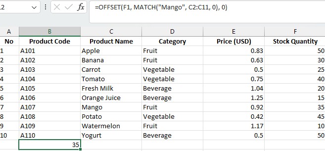
Example: Retrieve the stock quantity for “Mango”

=OFFSET(F1, MATCH("Mango", C2:C11, 0), 0)

Explanation:

• MATCH("Mango", C2:C11, 0) finds the row number of "Mango" (7th row).
• OFFSET(F1, 7, 0) moves 7 rows down in column E, retrieving the stock quantity.

Result: 35

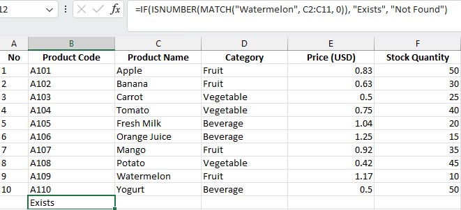
4️⃣ IF + ISNUMBER + MATCH (Check if a Value Exists in a List)

Why use this combination? This formula is used to check if a value exists in a list. If the value is found, it returns "Exists", otherwise "Not Found".

Example: Check if “Watermelon” is in the product list

=IF(ISNUMBER(MATCH("Watermelon", C2:C11, 0)), "Exists", "Not Found")

Explanation:

• MATCH("Watermelon", C2:C11, 0) searches for "Watermelon". If found, it returns a number (row index).
• ISNUMBER(...) checks if the MATCH  result is a valid number.
• IF(..., "Exists", "Not Found") returns "Exists" if MATCH  finds a match, otherwise "Not Found".

Result: "Exists"

Above is all you need to know about how to use the MATCH function in Excel. Although it is just a function to find a pair, not to calculate a value, it is extremely useful when you need to arrange data reasonably and logically.

Basically, using the Match function in Microsoft Excel is not too difficult if you grasp all the basic information above. Besides the Match function, Excel has many other useful functions. Let’s continue to learn about Excel functions with Lammoc in the following lessons!