The AGGREGATE function is a relatively complex function, but it is considered one of the most powerful Excel functions as it can replace multiple other functions. In this article, we will explore the power of the AGGREGATE function in Excel.
Nội dung
1. What is AGGREGATE?
The AGGREGATE function in Excel combines multiple functions into one and was introduced in Excel 2010. Since the AGGREGATE function has multiple options, it can be used as a substitute for functions such as SUM, COUNT, MAX, MIN, AVERAGE, LARGE, SMALL, and more. This makes AGGREGATE an extremely versatile function in Excel.
2. Syntax of the AGGREGATE Function
Reference Form Syntax:
=AGGREGATE(function_num, options, ref1, [ref2], …)
Array Form Syntax:
=AGGREGATE(function_num, options, array, [k])
Where:
- function_num: A number (1-19) that specifies the function to use, as shown in the table below.
- options: A number (0-7) that defines how AGGREGATE handles hidden rows and errors.
- ref1: The first value when multiple references are used.
- ref2, ref3,…ref253: Additional values to compute.
- array: The array to evaluate.
- k: The rank or position used for certain functions such as LARGE and SMALL.
Function Numbers and Their Corresponding Operations
| function_num | Function | Description | Form |
|---|---|---|---|
| 1 | AVERAGE | Calculates the average | Reference |
| 2 | COUNT | Counts the number of numeric values | Reference |
| 3 | COUNTA | Counts the number of non-empty cells | Reference |
| 4 | MAX | Returns the maximum value | Reference |
| 5 | MIN | Returns the minimum value | Reference |
| 6 | PRODUCT | Multiplies values together | Reference |
| 7 | STDEV.S | Estimates standard deviation based on a sample | Reference |
| 8 | STDEV.P | Computes the standard deviation based on a population | Reference |
| 9 | SUM | Sums up values | Reference |
| 10 | VAR.S | Estimates variance based on a sample | Reference |
| 11 | VAR.P | Computes variance based on a population | Reference |
| 12 | MEDIAN | Finds the median value | Reference |
| 13 | MODE.SNGL | Returns the most frequently occurring value | Reference |
| 14 | LARGE | Returns the nth largest value | Array |
| 15 | SMALL | Returns the nth smallest value | Array |
| 16 | PERCENTILE.INC | Returns the k-th percentile | Array |
| 17 | QUARTILE.INC | Returns the quartile | Array |
| 18 | PERCENTILE.EXC | Returns the k-th percentile | Array |
| 19 | QUARTILE.EXC | Returns the quartile | Array |
Options and Their Conditions
| options | Condition |
|---|---|
| 0 or empty | Ignores other SUBTOTAL or AGGREGATE functions |
| 1 | Ignores hidden rows and other SUBTOTAL or AGGREGATE functions |
| 2 | Ignores error values and other SUBTOTAL or AGGREGATE functions |
| 3 | Ignores hidden rows, error values, and other SUBTOTAL or AGGREGATE functions |
| 4 | Ignores empty rows |
| 5 | Ignores hidden rows |
| 6 | Ignores error values |
| 7 | Ignores hidden rows and error values |
Example Usage of AGGREGATE
AGGREGATE is often used to find the smallest or largest values in a dataset. For instance:
- The LARGE function returns the nth largest value in an array.
- The SMALL function returns the nth smallest value in an array.
Notes:
- When you type AGGREGATE in Excel, a list of
function_numandoptionswill appear, allowing you to select the appropriate number. - Leaving
ref1andref2empty may result in a#VALUEerror. - Functions such as
LARGE(array, k),SMALL(array, k),PERCENTILE.INC(array, k),QUARTILE.INC(array, quart),PERCENTILE.EXC(array, k), andQUARTILE.EXC(array, quart)require a second argument (k). - AGGREGATE calculates vertically. For example, using
function_num = 1in a horizontal range will not be affected by hidden columns, but hidden rows in a vertical range will impact the result. - The AGGREGATE function does not work with 3D references.
3. All Applications of the AGGREGATE function in Excel
Sample Data Table:
| Product | Quantity | Revenue |
|---|---|---|
| Milk | 50 | 2,500,000 |
| Cake | 30 | #DIV/0! |
| Pants | 20 | 3,500,000 |
| Shirt | 40 | 2,800,000 |
| Shoes | 25 | 2,300,000 |
| Sandals | 15 | #N/A |
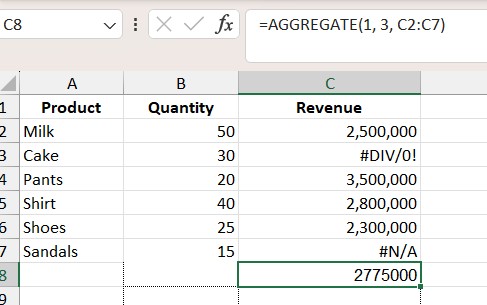
3.1. Calculate the Average While Ignoring Errors
Formula: =AGGREGATE(1, 3, C2:C7)
Explanation:
- 1: AVERAGE
- 3: Ignore errors (#DIV/0! and #N/A)
- C2:C7: Revenue column
Result: The average revenue excluding error values.
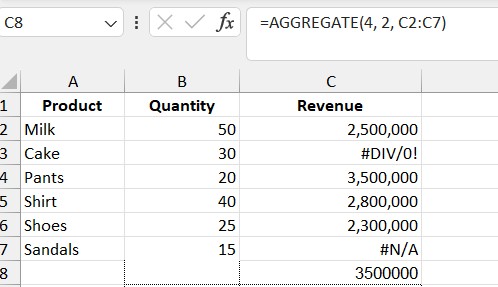
3.2. Find the Maximum Value While Ignoring Hidden Rows
Formula: =AGGREGATE(4, 2, C2:C7)
Explanation:
- 4: MAX
- 2: Ignore hidden rows
- C2:C7: Revenue column
Result: The highest revenue among non-hidden rows.
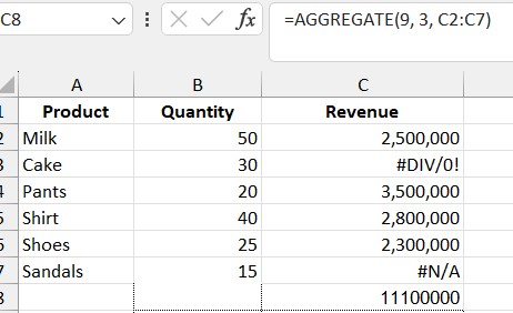
3.3. Calculate the Total While Ignoring Errors
Formula: =AGGREGATE(9, 3, C2:C7)
Explanation:
- 9: SUM
- 3: Ignore errors
- C2:C7: Revenue column
Result: The total revenue excluding error cells.
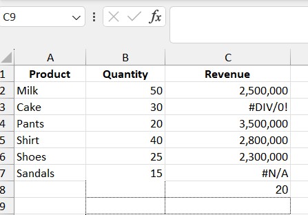
3.4. Find the 2nd Smallest Value
Formula: =AGGREGATE(15, 3, B2:B7, 2)
Explanation:
- 15: SMALL
- 3: Ignore errors
- B2:B7: Quantity column
- 2: The second smallest value
Result: 20 (since after 15, the next smallest value is 20 in the Quantity column).
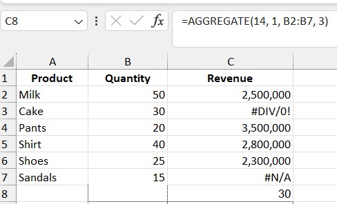
3.5. Find the 3rd Largest Value
Formula: =AGGREGATE(14, 1, B2:B7, 3)
Explanation:
- 14: LARGE
- 1: Ignore all hidden rows, errors, and hidden values
- B2:B7: Quantity column
- 3: The third largest value
Result: 30 (the third largest value after 50 and 40).
4. Comparison Between AGGREGATE and SUBTOTAL
| Criteria | AGGREGATE | SUBTOTAL |
|---|---|---|
| Number of Supported Functions | 19 | 11 |
| Ignore Errors | Yes | No |
| Find Large/Small K Values | Yes (LARGE, SMALL) | No |
| Flexibility in Calculations | High | Medium |
When to Use AGGREGATE?
- When you need to ignore errors.
- When finding large/small k values.
- When handling hidden data more flexibly than SUBTOTAL.
5. Conclusion
The AGGREGATE function in Excel is extremely versatile and powerful, especially useful when working with complex data sets that contain errors or hidden rows. Using the right function and parameters will help you process data more efficiently.
Try applying AGGREGATE today to enhance your Excel skills!
See more: Basic and Advanced DATE Function in Excel