OFFSET Function In Excel (Practical Application)

5

The OFFSET function in Excel is a powerful tool that allows users to reference cells dynamically without needing to specify their exact addresses. Instead of pointing to a fixed cell, the OFFSET function lets you move from an initial reference cell to a specific location based on the number of rows and columns, enabling flexible calculations and dynamic references. In this article, we will explore how to use the OFFSET function to optimize data processing and save time in handling complex calculations.

1. What is the OFFSET Function?

The OFFSET function in Excel helps reference a data range based on a starting cell and moves by a specified number of rows, columns, height, and width. This is a powerful tool for creating dynamic lists, flexible reports, and advanced data analysis.

Syntax:

OFFSET(reference, rows, cols, [height], [width])

• reference: The starting reference cell. (Required)
• rows: The number of rows to move from the reference. (Required)
• cols: The number of columns to move from the reference. (Required)
• height (Optional): The height (number of rows) of the returned range. (Optional)
• width (Optional): The width (number of columns) of the returned range. (Optional)

Key Highlights:

✅ Create dynamic lists: Automatically expands or contracts based on data changes.
✅ Flexible integration: Works well with functions like COUNTA, MATCH, INDEX, SUM, and AVERAGE.
✅ Customizable range selection: Easily adjust the height and width according to your needs.

Important Notes on Using the OFFSET Function in Excel

The OFFSET function helps reference a dynamic data range based on a starting position. When using this function, keep the following in mind:

Understanding the syntax:

OFFSET(reference, rows, cols, [height], [width])

• reference: The starting cell.
• rows, cols: The number of rows and columns to move.
• height, width (Optional): The size of the returned data range.

Best Practices:

Fix references properly: Use $ (absolute reference) to avoid errors when copying formulas.
Combine with other functions: OFFSET is most effective when used with COUNTA, MATCH, or COUNTIF.
Dynamic but not static: OFFSET updates automatically when data changes, but this can slow down large Excel files.
Check data limits: Avoid referencing beyond the spreadsheet range to prevent errors.

2. Use Cases of the OFFSET Function in Excel

Use Case	Description	Purpose
1. Create dynamic lists	Automatically updates the list when data is added/removed.	Reduces manual adjustments when data changes.
2. Create dependent lists	Displays data based on user selection (e.g., department, region).	Filters data according to user-defined criteria.
3. Create dynamic charts	Charts automatically expand when new data is added.	Updates charts without manually adjusting the range.
4. Reference flexible data ranges	Extracts data from a changing position without updating formulas.	Allows easy modification of the starting point and size.
5. Advanced data analysis	Defines data ranges for custom calculations.	Provides flexibility in analyzing large datasets.
6. Generate dynamic reports	Automatically updates report data based on input parameters.	Reduces the time spent modifying reports for each period.

3. Practical Applications of the OFFSET Function

3.1 Guide to Using the OFFSET Function to Create a Dynamic List in Excel

Create an Auto-Updating List Without Empty Rows at the End

Imagine you need to recruit 20 people for a team, but initially, you only have 5 employees. In a fixed list, empty rows will appear. As the number of employees changes over time, the list should automatically update without requiring manual adjustments.

Example Data Table

No	Name	Department
1	Nguyen Van A	Business
2	Tran Thi B	Business
3	Le Van C	Business
4	Pham Thi D	Accounting
5	Hoang Van E	Accounting
…	…	…
20	…	…

Step 1: Define the Starting Point

The starting point of the list can be determined in different ways:

Start at cell B2 and keep the row and column fixed.
Start at cell B1 and move down by one row.
Start at cell A1, move down one row, and move right one column.

Defining the starting point helps Excel understand where the list begins. This is crucial when combining OFFSET with other functions to expand the list dynamically.

For example, if the list starts at B3, the basic OFFSET formula would be:

=OFFSET(B2,0,0,row_count,column_count)

Step 2: Determine the List Length Using COUNTA

To determine the current number of employees in the list, use the COUNTA function to count the number of non-empty cells in column B from row 3 to row 22:

=COUNTA(B2:B20)

Example Results:
✔ If there are 5 employees, the result is 5.
✔ If there are 7 employees, the result is 7.

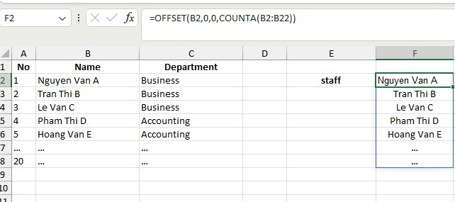
When integrated into the OFFSET function, the complete formula for creating a dynamic list is:

=OFFSET(B2,0,0,COUNTA(B2:B22))

Explanation of the Formula:

B2 is the starting cell.
0,0 keeps the row and column positions unchanged.
COUNTA(B2:B22) determines the number of rows with data.
No column parameter is needed, as the list is contained in a single column.

Step 3: Dynamic List Formula in Data Validation

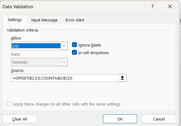
Once you have the correct OFFSET formula, you can use it to create a dynamic dropdown list in Excel through Data Validation:

=OFFSET(B2,0,0,COUNTA(B2:B22))

This formula ensures that only cells with data are included in the list while ignoring empty rows.

When new employees are added, the dropdown list automatically expands. For example, if two new employees are added to rows 6 and 7, the list will now contain 7 names instead of 5.

Steps to Enable Data Validation

1️⃣ Select the cell(s) or range where you want to create the dropdown list.
2️⃣ Go to the Data tab > Click Data Validation.
3️⃣ In the Allow field, choose List.
4️⃣ Enter the OFFSET formula into the Source field.
5️⃣ Click OK to apply.

Now, the dropdown list will automatically expand or shrink based on the number of employees, ensuring efficient data management without displaying empty rows.

3.2 Creating Dependent Dropdown Lists in Excel Using the OFFSET Function

In Excel, creating dependent dropdown lists allows data to be automatically filtered by category without manual selection. For example, you have a list of employees, each belonging to a different department such as Business or Accounting. When selecting a department, the employee list will only display those in the chosen department.

Example Data Table

List of Employees
No	Department	Name
1	Business	Nguyen Van A
2	Business	Tran Van B
3	Business	Le Thi C
4	Accounting	Dao Trung D
5	Accounting	Ngo Thi L
6	Accounting	Dao Van K
7	Accounting	Tran Tu A
…	…	…
20	…	…

To achieve this, we will use OFFSET combined with MATCH and COUNTIF to create a dynamic list.

Step 1: Identify the Starting Point of the List

First, we need to determine a fixed reference point. In this case, the employee list starts in column B. Let’s assume:

• Cell B2 contains the “Department” header.
• The employee list spans from B3 to B22.

The basic OFFSET formula to reference data from cell B2 is:

=OFFSET(B2, …)

Here, B2 serves as the reference point, allowing us to navigate dynamically to employees in the selected department.

Step 2: Find the Position of the Selected Department

Since employees belong to different departments, we need to determine the starting position of the selected department. The MATCH function helps locate its position in the list (B3:B22):

=MATCH(F2, B3:B22, 0)

Where:

• F2 contains the selected department (e.g., “Business” or “Accounting”).
• B3:B22 is the department column.

Example:

• Selecting "Business": The first occurrence is in B3 (row 1) → MATCH returns 1.
• Selecting "Accounting": The first occurrence is in B6 (row 4) → MATCH returns 4.

Now, integrating MATCH into OFFSET:

=OFFSET(B2, MATCH(F2, B3:B22, 0), …)

This formula moves to the first row of the selected department.

Step 3: Identify the Column Containing Employee Names

After locating the starting row, we need to extract employee names from column C (right next to column B). To move 1 column right, we modify the formula:

=OFFSET(B2, MATCH(F2, B3:B22, 0), 1, …)

Here, 1 represents shifting 1 column from B to C.

Step 4: Determine the Number of Rows to Extract (Employees in the Selected Department)

To count how many employees belong to the selected department, we use COUNTIF:

=COUNTIF(B3:B22, F2)

Example:

• Selecting "Business" → COUNTIF returns 3 (3 employees).
• Selecting "Accounting" → COUNTIF returns 4 (4 employees).

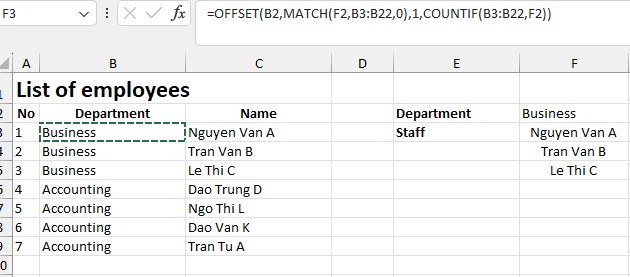
Now, integrating COUNTIF into OFFSET, we get the final formula:

=OFFSET(B2, MATCH(F2, B3:B22, 0), 1, COUNTIF(B3:B22, F2))

Where:

• MATCH(F2, B3:B22, 0) finds the starting row of the department.
• COUNTIF(B3:B22, F2) determines the number of employees in that department.

This formula dynamically extracts only the employees belonging to the selected department!

Step 5: Create a Dropdown List Using Data Validation

Now that we have the OFFSET formula, we can use it in Data Validation to create a dropdown list in cell F3.

Steps to Set Up Data Validation:

1. Select cell F3 (where the employee list will be displayed).
2. Go to the Data tab → Click Data Validation.
3. In the Data Validation window:
   • Under Allow, select List.
   • Under Source, enter the formula:

   =OFFSET($B$2,MATCH($F$2,$B$3:$B$22,0),1,COUNTIF($B$3:$B$22,$F$2))
   

4. Click OK to apply the settings.

Final Result:

✅ When selecting “Business” in F2, the dropdown in F3 will only show employees from the Business department.
✅ When selecting “Accounting” in F2, the list in F3 will automatically update to show only Accounting employees.

This method ensures that the dropdown dynamically updates based on the department selection, improving data accuracy and efficiency!

4. Why Use Data Validation When Creating Dynamic Lists in Excel?

1. Easily and Accurately Create Dropdown Lists

When combining Data Validation with the OFFSET function, you can create an automatically updating dropdown list without manual adjustments.

If data is added or removed from the source list, the dropdown in Data Validation will automatically update accordingly.

2. Prevent Data Entry Errors

Manual data entry can lead to typos or incorrect formatting.

With Data Validation, users can only select from predefined values, ensuring data accuracy and consistency.

3. Automatically Remove Blank Rows

If a dropdown list is created by selecting a fixed range, empty rows may appear in the list.

By using OFFSET + COUNTA in Data Validation, only cells with data are displayed, excluding empty cells.

4. Save Time and Improve Efficiency

When working with frequently changing data, using dynamic lists in Data Validation prevents the need for manual updates.

This is especially helpful when handling large datasets or Excel data entry forms.

5. Common Errors and How to Fix Them

Error	Cause	Solution
1. #REF! error appears	The rows or cols parameter exceeds the worksheet range.	Check the rows and cols values to ensure they stay within the sheet’s limits.
2. Formula does not return results	The height or width value is negative or not an integer.	Always use positive integers for height and width.
3. Dynamic list includes empty cells	The COUNTA function is used on a range containing empty cells.	Combine COUNTIF or FILTER to retrieve only the necessary data.
4. Incorrect results when copying the formula	Absolute references ($) are not used for the data range.	Add $ to fix references, e.g., $B$2.
5. Excel slows down or freezes	The OFFSET function recalculates continuously on large datasets.	Use INDEX instead of OFFSET if dynamic adjustment is unnecessary, or optimize the formula.
6. Data Validation does not show the list	The OFFSET formula is incorrectly entered in the Source field.	Ensure the formula is correct and references the right data range.

By using Data Validation effectively, you can ensure accuracy, efficiency, and better data management in Excel.

Conclusion

The OFFSET function is an invaluable tool in Excel that increases flexibility and efficiency when working with dynamic data. By allowing you to reference cells based on relative positions, it opens up new possibilities for complex calculations and data analysis. Mastering the OFFSET function in Excel can significantly streamline your workflow, allowing you to handle large data sets with ease and accuracy.
We encourage you to explore more advanced Excel functions and techniques in our upcoming articles to further enhance your skills and make your work even more efficient.

See more:
How to use MATCH Function in Excel (examples and function combinations)